Advanced HPC use cases
Overview
Teaching: 25 min
Exercises: 25 minQuestions
How can I run an MPI enabled application in a container using a bind approach?
How can I run a GPU enabled application in a container?
How can I store files inside a container filesystem?
How can I use workflow engines in conjunction with containers?
Objectives
Discuss the bind approach for containerised MPI applications, including its performance
Get started with containerised GPU applications
Run-real world MPI/GPU examples using OpenFoam and Gromacs
Run a data-intensive pipeline, saving data in an overlay filesystem
Get an idea of the interplay between containers and workflow engines
NOTE: the following hands-on session focuses on Singularity only.
Configure the MPI/interconnect bind approach
Before we start, let us cd to the openfoam example directory:
cd ~/sc-tutorials/exercises/openfoam
Now, suppose you have an MPI installation in your host and a containerised MPI application, built upon MPI libraries that are ABI compatible with the former.
For this tutorial, we do have MPICH installed on the host machine:
which mpirun
/opt/mvapich2-x/gnu11.1.0/mofed/aws/mpirun/bin/mpirun
and we’re going to pull an OpenFoam container, which was built on top of MPICH as well.
Since this is a large image, we will pull a copy to /tmp for everyone to share.
(cd /tmp && [ -e sc22-openfoam_v2012.sif ] || singularity pull docker://quay.io/pawsey/sc22-openfoam:v2012 && chmod a+r /tmp/sc22-openfoam_v2012.sif)
OpenFoam comes with a collection of executables, one of which is simpleFoam. We can use the Linux command ldd to investigate the libraries that this executable links to. As simpleFoam links to a few tens of libraries, let’s specifically look for MPI (libmpi*) libraries in the command output:
singularity exec /tmp/sc22-openfoam_v2012.sif bash -c 'ldd $(which simpleFoam) |grep libmpi'
libmpi.so.12 => /installs/lib/libmpi.so.12 (0x00007f3b982de000)
This is the container MPI installation that was used to build OpenFoam.
How do we setup a bind approach to make use of the host MPI installation?
We can make use of Singularity-specific environment variables, to make these host libraries available in the container (see location of MPICH from which mpirun above):
# We need to get the efa library
mkdir -p /tmp/lib
podman run -v /tmp/lib:/tmp/lib scanon/efalibraries:20.04
chmod a+rx -R /tmp/lib

export MPICH_ROOT="/opt/mvapich2-x/gnu11.1.0/mofed/aws/mpirun"
export SINGULARITY_BINDPATH="$MPICH_ROOT"
export SINGULARITYENV_LD_LIBRARY_PATH="$MPICH_ROOT/lib64:/tmp/lib:\$LD_LIBRARY_PATH"
Now, if we inspect mpirun dynamic linking again:
singularity exec /tmp/sc22-openfoam_v2012.sif bash -c 'ldd $(which simpleFoam) |grep libmpi'
libmpi.so.12 => /opt/mvapich2-x/gnu11.1.0/mofed/aws/mpirun/lib64/libmpi.so.12 (0x0000145ea2c00000)
Now OpenFoam is picking up the host MPI libraries!
Note that, on a HPC cluster, with the same mechanism it is possible to expose the host interconnect libraries in the container, to achieve maximum communication performance.
Let’s run OpenFoam in a container!
To get the real feeling of running an MPI application in a container, let’s run a practical example.
We’re using OpenFoam, a widely popular package for Computational Fluid Dynamics simulations, which is able to massively scale in parallel architectures up to thousands of processes, by leveraging an MPI library.
The sample inputs come straight from the OpenFoam installation tree, namely $FOAM_TUTORIALS/incompressible/pimpleFoam/LES/periodicHill/steadyState/.
Before getting started, let’s make sure that no previous output file is present in the exercise directory:
./clean-outputs.sh
Now, let’s execute the script in the current directory:
./mpirun_para.sh
This will take a few minutes to run. In the end, you will get the following output files/directories:
ls -ltr
total 1121572
-rwxr-xr-x. 1 tutorial livetau 1148433339 Nov  4 21:40 openfoam_v2012.sif
drwxr-xr-x. 2 tutorial livetau         59 Nov  4 21:57 0
-rw-r--r--. 1 tutorial livetau        798 Nov  4 21:57 slurm_pawsey.sh
-rwxr-xr-x. 1 tutorial livetau        843 Nov  4 21:57 mpirun.sh
-rwxr-xr-x. 1 tutorial livetau        197 Nov  4 21:57 clean-outputs.sh
-rwxr-xr-x. 1 tutorial livetau       1167 Nov  4 21:57 update-settings.sh
drwxr-xr-x. 2 tutorial livetau        141 Nov  4 21:57 system
drwxr-xr-x. 4 tutorial livetau         72 Nov  4 22:02 dynamicCode
drwxr-xr-x. 3 tutorial livetau         77 Nov  4 22:02 constant
-rw-r--r--. 1 tutorial livetau       3497 Nov  4 22:02 log.blockMesh
-rw-r--r--. 1 tutorial livetau       1941 Nov  4 22:03 log.topoSet
-rw-r--r--. 1 tutorial livetau       2304 Nov  4 22:03 log.decomposePar
drwxr-xr-x. 8 tutorial livetau         70 Nov  4 22:05 processor1
drwxr-xr-x. 8 tutorial livetau         70 Nov  4 22:05 processor0
-rw-r--r--. 1 tutorial livetau      18583 Nov  4 22:05 log.simpleFoam
drwxr-xr-x. 3 tutorial livetau         76 Nov  4 22:06 20
-rw-r--r--. 1 tutorial livetau       1533 Nov  4 22:06 log.reconstructPar
We ran using 2 MPI processes, who created outputs in the directories processor0 and processor1, respectively.
The final reconstruction creates results in the directory 20 (which stands for the 20th and last simulation step in this very short demo run), as well as the output file log.reconstructPar.
As execution proceeds, let’s ask ourselves: what does running singularity with MPI look run in the script? Here’s the script we’re executing:
#!/bin/bash

NTASKS="2"
#image="docker://quay.io/pawsey/sc22-openfoam:v2012"
image=/tmp/sc22-openfoam_v2012.sif

# this configuration depends on the host
export MPICH_ROOT="/opt/mvapich2-x/gnu11.1.0/mofed/aws/mpirun"
export MPICH_LIBS="$( which mpirun )"
export MPICH_LIBS="${MPICH_LIBS%/bin/mpirun*}/lib64/:/tmp/lib"

export SINGULARITY_BINDPATH="$MPICH_ROOT"
export SINGULARITYENV_LD_LIBRARY_PATH="$MPICH_LIBS:\$LD_LIBRARY_PATH"

# pre-processing
singularity exec $image \
  blockMesh | tee log.blockMesh

singularity exec $image \
  topoSet | tee log.topoSet

singularity exec $image \
  decomposePar -fileHandler uncollated | tee log.decomposePar


# run OpenFoam with MPI
mpirun -n $NTASKS \
  singularity exec $image \
  simpleFoam -fileHandler uncollated -parallel | tee log.simpleFoam


# post-processing
singularity exec $image \
  reconstructPar -latestTime -fileHandler uncollated | tee log.reconstructPar
In the beginning, Singularity variable SINGULARITY_BINDPATH and SINGULARITYENV_LD_LIBRARY_PATH are defined to setup the bind approach for MPI.
Then, a bunch of OpenFoam commands are executed, with only one being parallel:
mpirun -n $NTASKS \
  singularity exec $image \
  simpleFoam -fileHandler uncollated -parallel | tee log.simpleFoam
That’s as simple as prepending mpirun to the singularity command line, as for any other MPI application.
Singularity interface to Slurm
Now, have a look at the script variant for the Slurm scheduler, slurm_pawsey.sh:
srun -n $SLURM_NTASKS \
  singularity exec $image \
  simpleFoam -fileHandler uncollated -parallel | tee log.simpleFoam
The key difference is that every OpenFoam command is executed via srun, i.e. the Slurm wrapper for the MPI launcher, mpirun. Other schedulers will require a different command.
In practice, all we had to do was to replace mpirun with srun, as for any other MPI application.
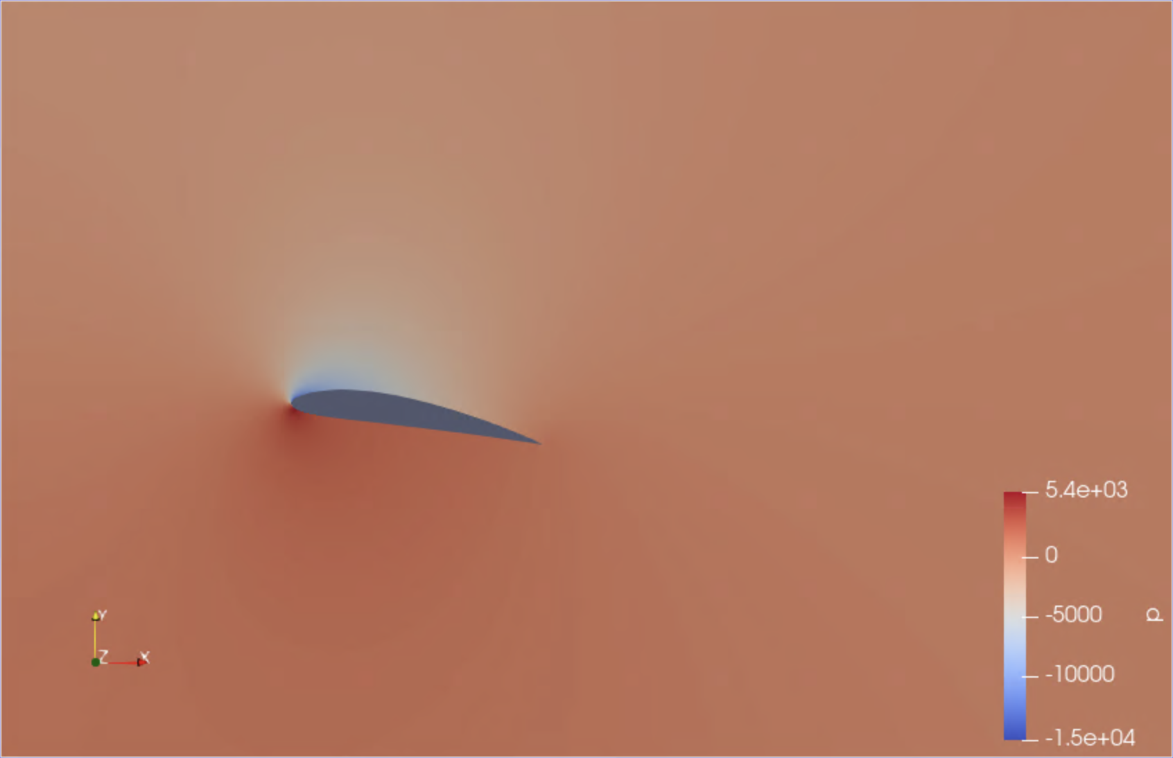
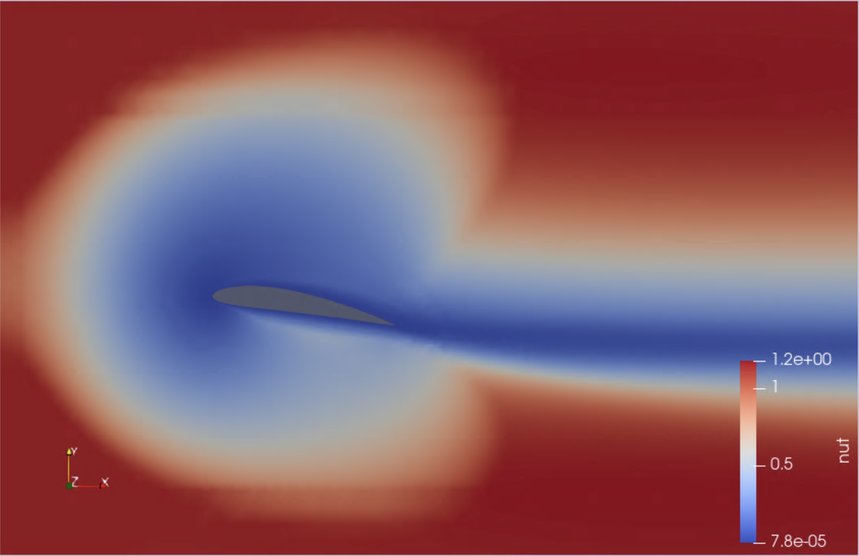
Bonus: a second OpenFoam example with visual output
If time allows, you may want to try out a second simulation, which models the air flow around a two-dimensional wing profile. This example has been kindly contributed by Alexis Espinosa at Pawsey Centre.
The required setup is as follows (a Slurm setup is also available in the alternate directory slurm_pawsey):
cd ~/sc-tutorials/exercises/openfoam_visual/mpirun
./mpirun.sh
This run uses 4 MPI processes and takes about 5-6 minutes. Upon completion, the file wingMotion2D_pimpleFoam/wingMotion2D_pimpleFoam.foam can be opened with the visualisation package Paraview, which is available for this training.
To launch Paraview, use your web browser to open the page https://tut<XXX>.supercontainers.org:8443/#e4s, and login with your training account details. Once you have got the Linux desktop, open up a terminal window and execute paraview. Use the File Open menu to find and open the .foam file mentioned above. Finally, follow the presenter’s instructions to visualise the simulation box. Here are a couple of snapshots:
 |
 |
|---|
We have just visualised the results of this containerised simulation!
DEMO: Container vs bare-metal MPI performance
NOTE: this part was executed on the Pawsey Zeus cluster. You can follow the outputs here.
Pawsey Centre provides a set of MPI base images, which also ship with the OSU Benchmark Suite. Let’s use it to get a feel of what it’s like to use or not to use the high-speed interconnect.
We’re going to run a small bandwidth benchmark using the image pawsey/mpich-base:3.1.4_ubuntu18.04. All of the required commands can be found in the directory path of the first OpenFoam example, in the script benchmark_pawsey.sh:
#!/bin/bash -l

#SBATCH --job-name=mpi
#SBATCH --nodes=2
#SBATCH --ntasks=2
#SBATCH --ntasks-per-node=1
#SBATCH --time=00:20:00
#SBATCH --output=benchmark_pawsey.out

image="docker://pawsey/mpich-base:3.1.4_ubuntu18.04"
osu_dir="/usr/local/libexec/osu-micro-benchmarks/mpi"

# this configuration depends on the host
module load singularity


# see that SINGULARITYENV_LD_LIBRARY_PATH is defined (host MPI/interconnect libraries)
echo $SINGULARITYENV_LD_LIBRARY_PATH

# 1st test, with host MPI/interconnect libraries
srun singularity exec $image \
  $osu_dir/pt2pt/osu_bw -m 1024:1048576


# unset SINGULARITYENV_LD_LIBRARY_PATH
unset SINGULARITYENV_LD_LIBRARY_PATH

# 2nd test, without host MPI/interconnect libraries
srun singularity exec $image \
  $osu_dir/pt2pt/osu_bw -m 1024:1048576
Basically we’re running the test twice, the first time using the full bind approach configuration as provided by the singularity module on the cluster, and the second time after unsetting the variable that makes the host MPI/interconnect libraries available in containers.
Here is the first output (using the interconnect):
# OSU MPI Bandwidth Test v5.4.1
# Size      Bandwidth (MB/s)
1024                 2281.94
2048                 3322.45
4096                 3976.66
8192                 5124.91
16384                5535.30
32768                5628.40
65536               10511.64
131072              11574.12
262144              11819.82
524288              11933.73
1048576             12035.23
And here is the second one:
# OSU MPI Bandwidth Test v5.4.1
# Size      Bandwidth (MB/s)
1024                   74.47
2048                   93.45
4096                  106.15
8192                  109.57
16384                 113.79
32768                 116.01
65536                 116.76
131072                116.82
262144                117.19
524288                117.37
1048576               117.44
Well, you can see that for a 1 MB message, the bandwidth is 12 GB/s versus 100 MB/s, quite a significant difference in performance!
DEMO: Run a molecular dynamics simulation on a GPU with containers
NOTE: this part was executed on the Pawsey Topaz cluster with Nvidia GPUs. You can follow the outputs here.
For our example we are going to use Gromacs, a quite popular molecular dynamics package, among the ones that have been optimised to run on GPUs through Nvidia containers.
To start, let us cd to the gromacs example directory:
cd ~/sc-tutorials/exercises/gromacs
This directory has got sample input files picked from the collection of Gromacs benchmark examples. In particular, we’re going to use the subset water-cut1.0_GMX50_bare/1536/.
Now, from a Singularity perspective, all we need to do to run a GPU application on Nvidia GPUs from a container is to add the runtime flag --nv. This will make Singularity look for the Nvidia drivers in the host, and mount them inside the container.
Then, on the host system side, when running GPU applications through Singularity the only requirement consists of the Nvidia driver for the relevant GPU card (the corresponding file is typically called libcuda.so.<VERSION> and is located in some library subdirectory of /usr).
Finally, GPU resources are usually made available in HPC systems through schedulers, to which Singularity natively and transparently interfaces. So, for instance let us have a look in the current directory at the Slurm batch script called gpu_pawsey.sh:
#!/bin/bash -l

#SBATCH --job-name=gpu
#SBATCH --partition=gpuq
#SBATCH --gres=gpu:1
#SBATCH --ntasks=1
#SBATCH --time=01:00:00
#SBATCH --output=gpu_pawsey.out

image="docker://nvcr.io/hpc/gromacs:2018.2"
module load singularity


# uncompress configuration input file
if [ -e conf.gro.gz ] ; then
 gunzip conf.gro.gz
fi


# run Gromacs preliminary step with container
srun singularity exec --nv $image \
    gmx grompp -f pme.mdp

# Run Gromacs MD with container
srun singularity exec --nv $image \
    gmx mdrun -ntmpi 1 -nb gpu -pin on -v -noconfout -nsteps 5000 -s topol.tpr -ntomp 1
Here, there are two key execution lines, who run a preliminary Gromacs job and the proper production job, respectively.
See how we have simply combined the Slurm command srun with singularity exec --nv <..> (similar to what we did in the episode on MPI):
srun singularity exec --nv $image gmx <..>
We can submit the script with:
sbatch gpu_pawsey.sh
A few files are produced, including the main output of the molecular dynamics run, md.log:
ls -ltr
total 139600
-rw-rw----+ 1 mdelapierre pawsey0001       664 Nov  5 14:07 topol.top
-rw-rw----+ 1 mdelapierre pawsey0001       950 Nov  5 14:07 rf.mdp
-rw-rw----+ 1 mdelapierre pawsey0001       939 Nov  5 14:07 pme.mdp
-rw-rw----+ 1 mdelapierre pawsey0001       556 Nov  5 14:07 gpu_pawsey.sh
-rw-rw----+ 1 mdelapierre pawsey0001 105984045 Nov  5 14:07 conf.gro
-rw-rw----+ 1 mdelapierre pawsey0001     11713 Nov  5 14:12 mdout.mdp
-rw-rw----+ 1 mdelapierre pawsey0001  36880760 Nov  5 14:12 topol.tpr
-rw-rw----+ 1 mdelapierre pawsey0001      9247 Nov  5 14:17 slurm-101713.out
-rw-rw----+ 1 mdelapierre pawsey0001     22768 Nov  5 14:17 md.log
-rw-rw----+ 1 mdelapierre pawsey0001      1152 Nov  5 14:17 ener.edr
Store the outputs of an RNA assembly pipeline inside an overlay filesystem using containers
There can be instances where, rather than reading/writing files in the host filesystem, it would instead come handy to persistently store them inside the container filesystem.
A practical user case is when using a host parallel filesystem such as Lustre to run applications that create a large number (e.g. millions) of small files. This practice creates a huge workload on the metadata servers of the filesystem, degrading its performance. In this context, significant performance benefits can be achieved by reading/writing these files inside the container.
Singularity offers a feature to achieve this, called OverlayFS.
Let us cd into the trinity example directory:
cd ~/sc-tutorials/exercises/trinity
And then execute the script run.sh:
./run.sh
It will run for a few minutes as we discuss its contents. The first part of the script defines the container image to be used for the analysis, and creates the filesystem-in-a-file:
#!/bin/bash

image="docker://trinityrnaseq/trinityrnaseq:2.8.6"

# create overlay
export COUNT="200"
export BS="1M"
export FILE="my_overlay"
singularity exec docker://ubuntu:18.04 bash -c " \
  mkdir -p overlay_tmp/upper overlay_tmp/work && \
  dd if=/dev/zero of=$FILE count=$COUNT bs=$BS && \
  mkfs.ext3 -d overlay_tmp $FILE && \
  rm -rf overlay_tmp"
Here, the Linux tools dd and mkfs.ext3 are used to create and format an empty ext3 filesystem in a file, which we are calling my_overlay. These Linux tools typically require sudo privileges to run. However, we can bypass this requirement by using the ones provided inside a standard Ubuntu container. This command looks a bit cumbersome, but is indeed just an idiomatic syntax to achieve our goal with Singularity (up to versions 3.7.x).
We have wrapped four commands into a single bash call from a container, just for the convenience of running it once. We’ve also defined shell variables for better clarity. What are the single commands doing?
We are creating (and then deleting at the end) two service directories, overlay_tmp/upper and overlay_tmp/work, that will be used by the command mkfs.ext3.
The dd command creates a file named my_overlay, made up of blocks of zeros, namely with count blocks of size bs (the unit here is megabytes); the product count*bs gives the total file size in bytes, in this case corresponding to 200 MB.
The command mkfs.ext3 is then used to format the file as a ext3 filesystem image, that will be usable by Singularity. Here we are using the service directory we created, my_overlay, with the flag -d, to tell mkfs we want the filesystem to be owned by the same owner of this directory, i.e. by the current user. If we skipped this option, we would end up with a filesystem that is writable only by root, not very useful.
Note how, starting from version 3.8, Singularity offers a dedicated syntax that wraps arounds the commands above, providing a simpler interface (here size must be in MB):
export SIZE="200"
export FILE="my_overlay"
singularity overlay create --size $SIZE $FILE
The second part uses the filesystem file we have just created. We are mounting it at container runtime by using the flag --overlay followed by the image filename, and then creating the directory /trinity_out_dir, which will be in the overlay filesystem:
# create output directory in overlay
OUTPUT_DIR="/trinity_out_dir"
singularity exec --overlay my_overlay docker://ubuntu:18.04 mkdir $OUTPUT_DIR
Finally, we are running the Trinity pipeline from the container, with the overlay filesystem mounted, and while telling Trinity to write the output in the directory we have just created:
# run analysis in overlay
singularity exec --overlay my_overlay $image \
  Trinity \
  --seqType fq --left trinity_test_data/reads.left.fq.gz  \
  --right trinity_test_data/reads.right.fq.gz \
  --max_memory 1G --CPU 1 --output $OUTPUT_DIR
When the execution finishes, we can inspect the outputs. Because these are stored in the OverlayFS, we need to use a Singularity container to inspect them:
singularity exec --overlay my_overlay docker://ubuntu:18.04 ls /trinity_out_dir
Trinity.fasta		      both.fa.read_count	       insilico_read_normalization   partitioned_reads.files.list.ok   recursive_trinity.cmds.ok
Trinity.fasta.gene_trans_map  chrysalis			       jellyfish.kmers.fa	     pipeliner.18881.cmds	       right.fa.ok
Trinity.timing		      inchworm.K25.L25.DS.fa	       jellyfish.kmers.fa.histo      read_partitions		       scaffolding_entries.sam
both.fa			      inchworm.K25.L25.DS.fa.finished  left.fa.ok		     recursive_trinity.cmds
both.fa.ok		      inchworm.kmer_count	       partitioned_reads.files.list  recursive_trinity.cmds.completed
Now let’s copy the assembled sequence and transcripts, Trinity.fasta*, in the current directory:
singularity exec --overlay my_overlay docker://ubuntu:18.04 bash -c 'cp -p /trinity_out_dir/Trinity.fasta* ./'
Note how we’re wrapping the copy command within bash -c; this is to defer the evaluation of the * wildcard to when the container runs the command.
We’ve run the entire workflow within the OverlayFS, and got only the two relevant output files out in the host filesystem!
ls -l Trinity.fasta*
-rw-r--r-- 1 ubuntu ubuntu 171507 Nov  4 05:49 Trinity.fasta
-rw-r--r-- 1 ubuntu ubuntu   2818 Nov  4 05:49 Trinity.fasta.gene_trans_map
Use scientific workflow engines using containerised software
Scientific workflow engines are particularly useful for data-intensive domains including (and not restricted to) bioinformatics and radioastronomy, where data analysis and processing is made up of a number of tasks to be repeatedly executed across large datasets. Some of the most popular ones, including Nextflow and Snakemake, provide interfaces to container engines. The combination of container and workflow engines can be very effective in enforcing reproducible, portable, scalable science.
Now, let’s try and use Singularity and Nextflow to run a demo RNA sequencing pipeline based on RNAseq-NF.
Let us cd into the nextflow example directory:
cd ~/sc-tutorials/exercises/nextflow
For convenience, a slightly edited version of the pipeline RNAseq-NF is already made available in this directory. This pipeline requires the bioinformatics packages called Salmon, FastQC and MultiQC. There are two critical files in here, namely main.nf, that contains the translation of the scientific pipeline in the Nextflow language, and nextflow.config, that contains several profiles for running with different software/hardware setups.
It’s time to launch the pipeline with Nextflow:
nextflow run main.nf
This run is failing with the following error:
[..]

Error executing process > 'index (ggal_1_48850000_49020000)'

Caused by:
  Process `index (ggal_1_48850000_49020000)` terminated with an error exit status (127)

Command executed:

  salmon index --threads 1 -t ggal_1_48850000_49020000.Ggal71.500bpflank.fa -i index

Command exit status:
  127

Command output:
  (empty)

Command error:
  .command.sh: line 2: salmon: command not found

[..]
This is the key snippet:
.command.sh: line 2: salmon: command not found
We don’t have the required packages .. let’s us containers then! To this end, we are going to activate one of the profiles that are available in nextflow.config, which is called singularity:
nextflow run main.nf -profile singularity
N E X T F L O W  ~  version 21.04.3
Launching `main.nf` [fabulous_yalow] - revision: b3e6e265f4
 R N A S E Q - N F   P I P E L I N E
 ===================================
 transcriptome: /home/tutorial/sc-tutorials/exercises/nextflow/data/ggal/ggal_1_48850000_49020000.Ggal71.500bpflank.fa
 reads        : /home/tutorial/sc-tutorials/exercises/nextflow/data/ggal/ggal_gut_{1,2}.fq
 outdir       : results

executor >  local (4)
[2f/9b131f] process > index (ggal_1_48850000_49020000) [100%] 1 of 1 ✔
[4e/3b378d] process > quant (ggal_gut)                 [100%] 1 of 1 ✔
[fa/701646] process > fastqc (FASTQC on ggal_gut)      [100%] 1 of 1 ✔
[89/cf4788] process > multiqc                          [100%] 1 of 1 ✔

Done! Open the following report in your browser --> results/multiqc_report.html
The pipeline has now run! The final output of this pipeline is an HTML report of a quality control task, which you might eventually want to download and open up in your browser.
However, the key question here is: how could the sole flag -profile singularity trigger the containerised execution? This is the relevant snippet from the nextflow.config file:
  singularity {
    process.container = 'nextflow/rnaseq-nf:latest'
    singularity.autoMounts = true
    singularity.cacheDir = "$NXF_HOME/singularity"
    singularity.enabled = true
  }
The image name is specified using the process.container keyword. Also, singularity.autoMounts is required to have the directory paths with the input files automatically bind mounted in the container. To save the time of pulling the image, we’re specifying a location for cached container images using singularity.cacheDir. Finally, singularity.enabled triggers the use of Singularity.
Based on this configuration file, Nextflow is able to handle all of the relevant Singularity commands by itself, i.e. pull and exec with the appropriate flags, such as -B for bind mounting host directories. In this case, as a user you don’t need to know in detail the Singularity syntax, but just the name of the container!
More information on configuring Nextflow to run Singularity containers can be found at Singularity containers.
Key Points
Appropriate Singularity environment variables can be used to configure the bind approach for MPI containers (sys admins can help); Shifter achieves this via a configuration file
Singularity and Shifter interface almost transparently with HPC schedulers such as Slurm
MPI performance of containerised applications almost coincide with those of a native run
You can run containerised GPU applications with Singularity using the flags
--nvor--rocmfor Nvidia or AMD GPUs, respectivelySingularity and Shifter allow creating and using filesystems-in-a-file, leveraging the OverlayFS technology
Mount an overlay filesystem with Singularity using the flag
--overlay <filename>Some workflow engines offer transparent APIs for running containerised applications
If you need to run data analysis pipelines, the combination of containers and workflow engines can really make your life easier!